The ISNUMBER function in Microsoft Excel is an information function that checks whether a given value is there inside a particular cell or not. This works for both texts as well as numbers and returns a value of TRUE or FALSE.
Though this is a very simple function, it can be used with a combination of other functions like Search, if, etc. to generate complex algorithms and use them in Excel. If used alone, the ISNUMBER function lets you test the value available inside a cell or a group of cells.
How to use the ISNUMBER function in Excel
The ISNUMBER function in Excel lets you perform conditional formatting on Cells (having Numbers) and determine if that value is achieved. Say, for example, you want a Cell to fill only in cases where it is a Number.
Using this ISNUMBER function, you may put some conditions under which this returns a logical value of TRUE if the value is a number, and FALSE if it is not. To use this function on Microsoft Excel, do the following –
- First of all, open a new or existing Excel spreadsheet.
- Now, pick the cell where you would like to have the result of this function.
- Type the following on this cell and replace the value under brackets with the cell reference or the value you want to test.
=ISNUMBER(value)
- Say, for example, you want to check if a particular Cell is having some numbers or not, use this code –
=ISNUMBER(C5)
- Press Enter and you will see TRUE appearing on it if there is some number inside that Cell.
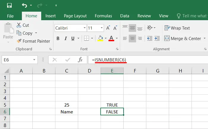
- This will return a FALSE value if there is something else inside that particular cell.
Users may also use this ISNUMBER function in combination with the IF function to perform conditional formatting. This function can also be used with some other functions to create some complex formulae.
Fix Microsoft Excel is too slow in Windows 11/10
How to find this ISNUMBER function in Excel
To use this function in Excel, you may try out either of the following three ways. However, before you do anything, make sure to select the specific Cell where you would like to see the result. Assuming you have already selected a Cell, now do the following –
- On the Cell itself, start typing “=ISNUMBER()” without quotes.
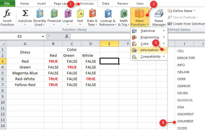
- Go to the Formulas tab and select More functions. When a drop-down menu appears, click Information > ISNUMBER.
- Alternatively, one may also use this ISNUMBER function using the fx key. See the Snapshot below –
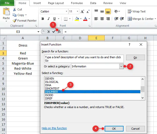
When the function arguments open, type the ISNUMBER function starting with the “=” icon and the argument that you would like to look up. Click OK and you will see the result in the selected Cell.
How do I use ISNUMBER in conditional formatting?
As stated above, one can use this ISNUMBER function in Excel to perform some conditional formatting. Well, here’s how –
- First of all, launch Microsoft Excel and fill in all your necessary data.
- Select all the cells to which you would like to apply conditional formatting.
- Now, go to the Home tab and click the Conditional Formatting button under Styles.
- When a drop-down menu opens up, select New Rule.
- You will now be redirected to a new window that contains applying six different rules.
- Select the Rule type “Use a formula to determine which cells to format.“
- Type the following in the Format values where this formula is true. See the Snapshot below –
=ISNUMBER(SEARCH ("RED", $A3))
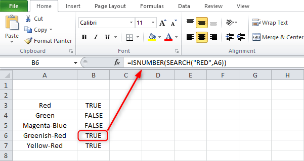
- The above formula works fine for a single cell. However, if you have a sample of data, you need to modify this formula every time you want to use it.
- Well, there’s a solution to this. Make a list of all colors in the adjacent columns and use this formula instead.
=ISNUMBER(SEARCH(C$2,$A4))
- In the above formula, C$2 represents the color that you would like to search for and $A4 is the Cell where you would like to search. Change these cell numbers as per your need.

- Press Enter and you will see the result accordingly.
How do I color format the results of the ISNUMBER function?
If you want to change the ISNUMBER function result’s color i.e. TRUE appearing differently, do the following –
- First of all, select all the Cells in which the TRUE or FALSE is going to appear.
- Now, click Conditional Formatting under Styles and choose New Rule.
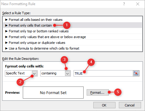
- Select the second rule i.e. Format only cells that contain. Under the Edit the Rule Description, select Specific Text, Containing, and write down TRUE in the text field. See the Snapshot below –
- Click Format and in the next window, choose a color using the drop-down menu.
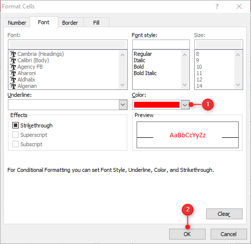
- Click OK and you will see all Cells having the TRUE as a result will now turn Red (the chosen color).
How do I find a text or a number in Excel?
There are times when you want to search for a particular text or number in the excel spreadsheet. If your excel file doesn’t have large information, you may find that value quite easily. However, this becomes tricky if you have a huge array of data.
Well, in that case, you may press Ctrl + F, and type “to be searched item” under the “Find what:” section. Click Find All so that you get each instance of the searched text or number.
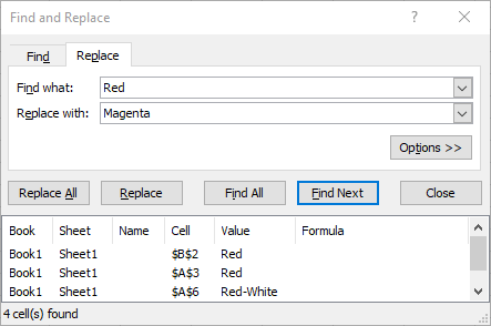
The first of all cells where the searched item is found will be highlighted automatically. In case you would like to replace the searched text with some other text, go to the Replace tab, and type the same under “Replace with:“.
Click Replace if you would like to change a cell only. To change all values bearing the searched-in info, click Replace all. Wait for a few seconds and Excel will replace the chosen text with your preferred text.
That’s it.


